Dda Circle Drawing Algorithm in Computer Graphics With Example

Selects raster points to course a close approximation to a straight line segment

Bresenham's line algorithm is a line drawing algorithm that determines the points of an north-dimensional raster that should be selected in order to form a close approximation to a straight line betwixt ii points. It is commonly used to draw line primitives in a bitmap image (e.g. on a computer screen), equally it uses but integer addition, subtraction and scrap shifting, all of which are very cheap operations in commonly used calculator instruction sets such as x86_64. It is an incremental error algorithm. It is ane of the primeval algorithms adult in the field of calculator graphics. An extension to the original algorithm may be used for drawing circles.

While algorithms such as Wu'southward algorithm are also frequently used in mod figurer graphics because they can support antialiasing, the speed and simplicity of Bresenham's line algorithm means that it is still important. The algorithm is used in hardware such as plotters and in the graphics chips of modern graphics cards. It can also be found in many software graphics libraries. Considering the algorithm is very simple, information technology is oft implemented in either the firmware or the graphics hardware of modern graphics cards.

The label "Bresenham" is used today for a family of algorithms extending or modifying Bresenham'south original algorithm.

History [edit]

Bresenham's line algorithm is named after Jack Elton Bresenham who developed it in 1962 at IBM. In 2001 Bresenham wrote:^[1]

I was working in the computation lab at IBM'southward San Jose development lab. A Calcomp plotter had been attached to an IBM 1401 via the 1407 typewriter panel. [The algorithm] was in production use past summertime 1962, possibly a month or so before. Programs in those days were freely exchanged among corporations so Calcomp (Jim Newland and Calvin Hefte) had copies. When I returned to Stanford in Fall 1962, I put a copy in the Stanford comp center library. A description of the line drawing routine was accepted for presentation at the 1963 ACM national convention in Denver, Colorado. It was a year in which no proceedings were published, only the agenda of speakers and topics in an issue of Communications of the ACM. A person from the IBM Systems Journal asked me after I fabricated my presentation if they could publish the paper. I happily agreed, and they printed it in 1965.

Bresenham'due south algorithm has been extended to produce circles, ellipses, cubic and quadratic bezier curves, as well as native anti-aliased versions of those.^[two]

Method [edit]

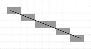
Illustration of the outcome of Bresenham'south line algorithm. (0,0) is at the top left corner of the grid, (1,1) is at the acme left end of the line and (xi, 5) is at the bottom right terminate of the line.

The following conventions will be used:

• the top-left is (0,0) such that pixel coordinates increase in the right and downward directions (eastward.yard. that the pixel at (7,iv) is directly above the pixel at (vii,5)), and
• the pixel centers have integer coordinates.

The endpoints of the line are the pixels at ${\displaystyle (x_{0},y_{0})}$ and ${\displaystyle (x_{1},y_{ane})}$ , where the kickoff coordinate of the pair is the cavalcade and the second is the row.

The algorithm will be initially presented simply for the octant in which the segment goes downwards and to the right ( ${\displaystyle x_{0}\leq x_{one}}$ and ${\displaystyle y_{0}\leq y_{i}}$ ), and its horizontal projection ${\displaystyle x_{1}-x_{0}}$ is longer than the vertical projection ${\displaystyle y_{i}-y_{0}}$ (the line has a positive gradient less than ane). In this octant, for each column x between ${\displaystyle x_{0}}$ and ${\displaystyle x_{1}}$ , there is exactly one row y (computed past the algorithm) containing a pixel of the line, while each row between ${\displaystyle y_{0}}$ and ${\displaystyle y_{i}}$ may contain multiple rasterized pixels.

Bresenham's algorithm chooses the integer y corresponding to the pixel center that is closest to the ideal (fractional) y for the same x; on successive columns y tin can remain the aforementioned or increase by i. The full general equation of the line through the endpoints is given by:

${\displaystyle {\frac {y-y_{0}}{y_{1}-y_{0}}}={\frac {x-x_{0}}{x_{i}-x_{0}}}}$ .

Since we know the column, x, the pixel's row, y, is given past rounding this quantity to the nearest integer:

${\displaystyle y={\frac {y_{1}-y_{0}}{x_{ane}-x_{0}}}(x-x_{0})+y_{0}}$ .

The gradient ${\displaystyle (y_{1}-y_{0})/(x_{1}-x_{0})}$ depends on the endpoint coordinates only and can exist precomputed, and the ideal y for successive integer values of 10 tin can be computed starting from ${\displaystyle y_{0}}$ and repeatedly adding the slope.

In practice, the algorithm does not continue track of the y coordinate, which increases past m = ∆y/∆x each time the 10 increases by one; it keeps an error spring at each stage, which represents the negative of the distance from (a) the point where the line exits the pixel to (b) the top border of the pixel. This value is first set to ${\displaystyle y_{0}-0.5}$ (due to using the pixel'southward centre coordinates), and is incremented by m each time the x coordinate is incremented by one. If the mistake becomes greater than 0.5, we know that the line has moved up 1 pixel, and that nosotros must increment our y coordinate and readjust the error to represent the distance from the top of the new pixel – which is done by subtracting one from error. ^[iii]

Derivation [edit]

To derive Bresenham'due south algorithm, two steps must exist taken. The get-go step is transforming the equation of a line from the typical slope-intercept form into something different; and then using this new equation to draw a line based on the idea of accumulation of error.

Line equation [edit]

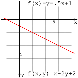
y=f(x)=.5x+1 or f(x,y)=x-2y+2

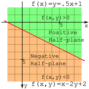
Positive and negative half-planes

The slope-intercept form of a line is written as

${\displaystyle y=f(x)=mx+b}$

where m is the gradient and b is the y-intercept. This is a part of only x and it would exist useful to make this equation written as a office of both x and y. Using algebraic manipulation and recognition that the slope is the "rise over run" or ${\displaystyle \Delta y/\Delta x}$ and then

${\displaystyle {\begin{aligned}y&=mx+b\\y&={\frac {(\Delta y)}{(\Delta x)}}ten+b\\(\Delta x)y&=(\Delta y)x+(\Delta x)b\\0&=(\Delta y)x-(\Delta x)y+(\Delta 10)b\terminate{aligned}}}$

Letting this final equation be a function of x and y and so it can be written as

${\displaystyle f(x,y)=0=Ax+By+C}$

where the constants are

The line is then defined for some constants A, B, and C anywhere ${\displaystyle f(x,y)=0}$ . For any ${\displaystyle (x,y)}$ not on the line then ${\displaystyle f(x,y)\neq 0}$ . Everything about this form involves merely integers if x and y are integers since the constants are necessarily integers.

As an case, the line ${\displaystyle y={\frac {i}{2}}10+1}$ and so this could be written as ${\displaystyle f(10,y)=ten-2y+two}$ . The signal (2,2) is on the line

${\displaystyle f(2,ii)=x-2y+2=(2)-2(two)+2=ii-4+two=0}$

and the signal (2,iii) is not on the line

${\displaystyle f(ii,three)=(2)-2(three)+two=2-six+two=-two}$

and neither is the point (2,1)

${\displaystyle f(2,1)=(2)-two(1)+two=2-2+2=2}$

Discover that the points (two,1) and (two,three) are on contrary sides of the line and f(ten,y) evaluates to positive or negative. A line splits a airplane into halves and the one-half-plane that has a negative f(10,y) tin exist called the negative half-aeroplane, and the other half can be called the positive half-plane. This observation is very of import in the remainder of the derivation.

Algorithm [edit]

Clearly, the starting point is on the line

${\displaystyle f(x_{0},y_{0})=0}$

but because the line is defined to start and end on integer coordinates (though it is entirely reasonable to want to draw a line with non-integer cease points).

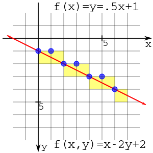
Candidate point (2,2) in blue and ii candidate points in light-green (three,ii) and (3,iii)

Keeping in listen that the gradient is at virtually ${\displaystyle 1}$ , the problem now presents itself equally to whether the next betoken should be at ${\displaystyle (x_{0}+one,y_{0})}$ or ${\displaystyle (x_{0}+1,y_{0}+ane)}$ . Maybe intuitively, the signal should be chosen based upon which is closer to the line at ${\displaystyle x_{0}+1}$ . If it is closer to the former then include the erstwhile betoken on the line, if the latter so the latter. To answer this, evaluate the line function at the midpoint betwixt these two points:

${\displaystyle f(x_{0}+1,y_{0}+{\tfrac {ane}{ii}})}$

If the value of this is positive and so the platonic line is below the midpoint and closer to the candidate indicate ${\displaystyle (x_{0}+1,y_{0}+one)}$ ; in consequence the y coordinate has advanced. Otherwise, the platonic line passes through or above the midpoint, and the y coordinate has not advanced; in this case choose the indicate ${\displaystyle (x_{0}+1,y_{0})}$ . This ascertainment is crucial to understand! The value of the line office at this midpoint is the sole determinant of which bespeak should be chosen.

The next epitome shows the blue bespeak (2,2) chosen to be on the line with two candidate points in dark-green (three,2) and (3,3). The black point (three, 2.5) is the midpoint between the two candidate points.

Algorithm for integer arithmetics [edit]

Alternatively, the deviation between points can be used instead of evaluating f(x,y) at midpoints. This alternative method allows for integer-only arithmetic, which is generally faster than using floating-betoken arithmetic. To derive the alternative method, define the divergence to be as follows:

${\displaystyle D=f(x_{0}+1,y_{0}+{\tfrac {one}{2}})-f(x_{0},y_{0})}$

For the first decision, this formulation is equivalent to the midpoint method since ${\displaystyle f(x_{0},y_{0})=0}$ at the starting point. Simplifying this expression yields:

${\displaystyle {\begin{array}{rclcl}D&=&\left[A(x_{0}+ane)+B\left(y_{0}+{\frac {one}{2}}\correct)+C\correct]&-&\left[Ax_{0}+By_{0}+C\correct]\\&=&\left[Ax_{0}+By_{0}+C+A+{\frac {1}{two}}B\right]&-&\left[Ax_{0}+By_{0}+C\right]\\&=&A+{\frac {1}{2}}B=\Delta y-{\frac {1}{2}}\Delta ten\end{array}}}$

Just as with the midpoint method, if ${\displaystyle D}$ is positive, and so choose ${\displaystyle (x_{0}+one,y_{0}+1)}$ , otherwise cull ${\displaystyle (x_{0}+ane,y_{0})}$ .

If ${\displaystyle (x_{0}+1,y_{0})}$ is chosen, the change in D will be:

${\displaystyle {\begin{array}{lclcl}\Delta D&=&f(x_{0}+2,y_{0}+{\tfrac {1}{2}})-f(x_{0}+i,y_{0}+{\tfrac {1}{ii}})&=&A&=&\Delta y\\\end{array}}}$

If ${\displaystyle (x_{0}+1,y_{0}+i)}$ is chosen the change in D will be:

${\displaystyle {\begin{array}{lclcl}\Delta D&=&f(x_{0}+two,y_{0}+{\tfrac {3}{2}})-f(x_{0}+1,y_{0}+{\tfrac {1}{2}})&=&A+B&=&\Delta y-\Delta x\end{array}}}$

If the new D is positive then ${\displaystyle (x_{0}+2,y_{0}+one)}$ is chosen, otherwise ${\displaystyle (x_{0}+2,y_{0})}$ . This decision can exist generalized past accumulating the error on each subsequent point.

Plotting the line from (0,1) to (6,4) showing a plot of grid lines and pixels

All of the derivation for the algorithm is done. One performance issue is the 1/two factor in the initial value of D. Since all of this is almost the sign of the accumulated departure, so everything tin can be multiplied by 2 with no consequence.

This results in an algorithm that uses simply integer arithmetic.

plotLine(x0, y0, x1, y1)     dx = x1 - x0     dy = y1 - y0     D = 2*dy - dx     y = y0          for          10 from x0 to x1         plot(ten,y)          if          D > 0             y = y + 1             D = D - two*dx          end if          D = D + 2*dy        

Running this algorithm for ${\displaystyle f(x,y)=x-2y+2}$ from (0,1) to (6,iv) yields the post-obit differences with dx=6 and dy=3:

D=ii*3-vi=0 Loop from 0 to 6  * x=0:          plot(0, 1), D≤0: D=0+6=six  * x=1:          plot(1, 1), D>0: D=6-12=-vi, y=1+i=two, D=-6+6=0  * x=2:          plot(ii, 2), D≤0: D=0+half-dozen=half-dozen  * x=3:          plot(3, 2), D>0: D=half dozen-12=-six, y=2+1=three, D=-vi+half-dozen=0  * x=4:          plot(iv, iii), D≤0: D=0+6=6  * x=5:          plot(5, iii), D>0: D=six-12=-6, y=three+1=four, D=-half dozen+6=0  * x=6:          plot(6, 4), D≤0: D=0+vi=6        

The result of this plot is shown to the right. The plotting can be viewed by plotting at the intersection of lines (blueish circles) or filling in pixel boxes (yellow squares). Regardless, the plotting is the same.

All cases [edit]

Still, equally mentioned above this is only for octant zero, that is lines starting at the origin with a slope between 0 and one where x increases past exactly one per iteration and y increases by 0 or 1.

The algorithm can be extended to cover slopes between 0 and -1 by checking whether y needs to increase or decrease (i.eastward. dy < 0)

plotLineLow(x0, y0, x1, y1)     dx = x1 - x0     dy = y1 - y0     yi = 1          if          dy < 0         yi = -1         dy = -dy          end if          D = (2 * dy) - dx     y = y0          for          x from x0 to x1         plot(ten, y)          if          D > 0             y = y + yi             D = D + (ii * (dy - dx))          else          D = D + two*dy          end if        

By switching the x and y axis an implementation for positive or negative steep slopes can exist written as

plotLineHigh(x0, y0, x1, y1)     dx = x1 - x0     dy = y1 - y0     xi = 1          if          dx < 0         xi = -one         dx = -dx          end if          D = (2 * dx) - dy     x = x0          for          y from y0 to y1         plot(10, y)          if          D > 0             ten = x + eleven             D = D + (2 * (dx - dy))          else          D = D + two*dx          end if        

A complete solution would need to find whether x1 > x0 or y1 > y0 and reverse the input coordinates earlier drawing, thus

plotLine(x0, y0, x1, y1)          if          abs(y1 - y0) < abs(x1 - x0)          if          x0 > x1             plotLineLow(x1, y1, x0, y0)          else          plotLineLow(x0, y0, x1, y1)          end if          else          if          y0 > y1             plotLineHigh(x1, y1, x0, y0)          else          plotLineHigh(x0, y0, x1, y1)          end if          end if        

In low level implementations which access the video memory directly, it would be typical for the special cases of vertical and horizontal lines to be handled separately as they can be highly optimized.

Some versions utilise Bresenham's principles of integer incremental fault to perform all octant line draws, balancing the positive and negative fault between the x and y coordinates.^[2] Take note that the club is non necessarily guaranteed; in other words, the line may be drawn from (x0, y0) to (x1, y1) or from (x1, y1) to (x0, y0).

plotLine(x0, y0, x1, y1)     dx = abs(x1 - x0)     sx = x0 < x1 ? 1 : -i     dy = -abs(y1 - y0)     sy = y0 < y1 ? i : -ane     mistake = dx + dy          while          truthful         plot(x0, y0)          if          x0 == x1 && y0 == y1          break          e2 = ii * mistake          if          e2 >= dy          if          x0 == x1          break          error = error + dy             x0 = x0 + sx          end if          if          e2 <= dx          if          y0 == y1          suspension          error = error + dx             y0 = y0 + sy          terminate if          end while        

Similar algorithms [edit]

The Bresenham algorithm can be interpreted as slightly modified digital differential analyzer (using 0.5 equally error threshold instead of 0, which is required for not-overlapping polygon rasterizing).

The principle of using an incremental fault in identify of division operations has other applications in graphics. It is possible to utilise this technique to summate the U,Five co-ordinates during raster browse of texture mapped polygons.^[4] The voxel heightmap software-rendering engines seen in some PC games also used this principle.

Bresenham besides published a Run-Slice (equally opposed to the Run-Length) computational algorithm. This method has been represented in a number of US patents:

5,815,163		Method and apparatus to draw line slices during calculation
five,740,345		Method and apparatus for displaying computer graphics data stored in a compressed format with an efficient color indexing system
v,657,435		Run slice line draw engine with non-linear scaling capabilities
five,627,957		Run slice line draw engine with enhanced processing capabilities
v,627,956		Run slice line draw engine with stretching capabilities
five,617,524		Run piece line draw engine with shading capabilities
5,611,029		Run slice line draw engine with non-linear shading capabilities
5,604,852		Method and apparatus for displaying a parametric curve on a video brandish
5,600,769		Run piece line draw engine with enhanced clipping techniques

An extension to the algorithm that handles thick lines was created by Alan Irish potato at IBM.^[v]

See also [edit]

• Digital differential analyzer (graphics algorithm), a simple and full general method for rasterizing lines and triangles
• Xiaolin Wu's line algorithm, a similarly fast method of cartoon lines with antialiasing
• Midpoint circle algorithm, a similar algorithm for cartoon circles

Notes [edit]

1. ^ Paul E. Black. Dictionary of Algorithms and Data Structures, NIST. https://xlinux.nist.gov/dads/HTML/bresenham.html
2. ^ ^{a b} Zingl, Alois "A Rasterizing Algorithm for Drawing Curves" (2012) http://members.chello.at/~easyfilter/Bresenham.pdf
3. ^ Joy, Kenneth. "Bresenham's Algorithm" (PDF). Visualization and Graphics Research Group, Department of Reckoner Science, Academy of California, Davis. Retrieved 20 December 2016.
4. ^ US 5739818, Spackman, John Neil, "Apparatus and method for performing perspectively correct interpolation in figurer graphics", published 1998-04-14, assigned to Canon KK
5. ^ "Murphy'southward Modified Bresenham Line Algorithm". homepages.enterprise.cyberspace . Retrieved 2018-06-09 .

References [edit]

• Bresenham, J. East. (1965). "Algorithm for computer control of a digital plotter" (PDF). IBM Systems Journal. 4 (1): 25–30. doi:x.1147/sj.41.0025. Archived from the original (PDF) on May 28, 2008.
• "The Bresenham Line-Drawing Algorithm", by Colin Flanagan
• Abrash, Michael (1997). Michael Abrash's graphics programming blackness volume . Albany, NY: Coriolis. pp. 654–678. ISBN978-1-57610-174-2. A very optimized version of the algorithm in C and assembly for use in video games with complete details of its inner workings
• Zingl, Alois (2012). "A Rasterizing Algorithm for Drawing Curves" (PDF). , The Beauty of Bresenham'southward Algorithms

Further reading [edit]

• Patrick-Gilles Maillot's Thesis an extension of the Bresenham line drawing algorithm to perform 3D hidden lines removal; likewise published in MICAD '87 proceedings on CAD/CAM and Computer Graphics, folio 591 - ISBN 2-86601-084-1.
• Line Thickening by Modification To Bresenham'south Algorithm, A.S. Murphy, IBM Technical Disclosure Bulletin, Vol. twenty, No. 12, May 1978.

rather than [which] for circle extension utilize: Technical Report 1964 January-27 -11- Circle Algorithm TR-02-286 IBM San Jose Lab or A Linear Algorithm for Incremental Digital Display of Circular Arcs February 1977 Communications of the ACM xx(2):100-106 DOI:x.1145/359423.359432

External links [edit]

• Michael Abrash'due south Graphics Programming Black Volume Special Edition: Chapter 35: Bresenham Is Fast, and Fast Is Good
• The Bresenham Line-Drawing Algorithm by Colin Flanagan
• National Plant of Standards and Applied science page on Bresenham's algorithm
• Calcomp 563 Incremental Plotter Information
• Bresenham Algorithm in several programming languages
• The Beauty of Bresenham's Algorithm – A elementary implementation to plot lines, circles, ellipses and Bézier curves

friedmancourel.blogspot.com

Source: https://en.wikipedia.org/wiki/Bresenham%27s_line_algorithm

Share this post